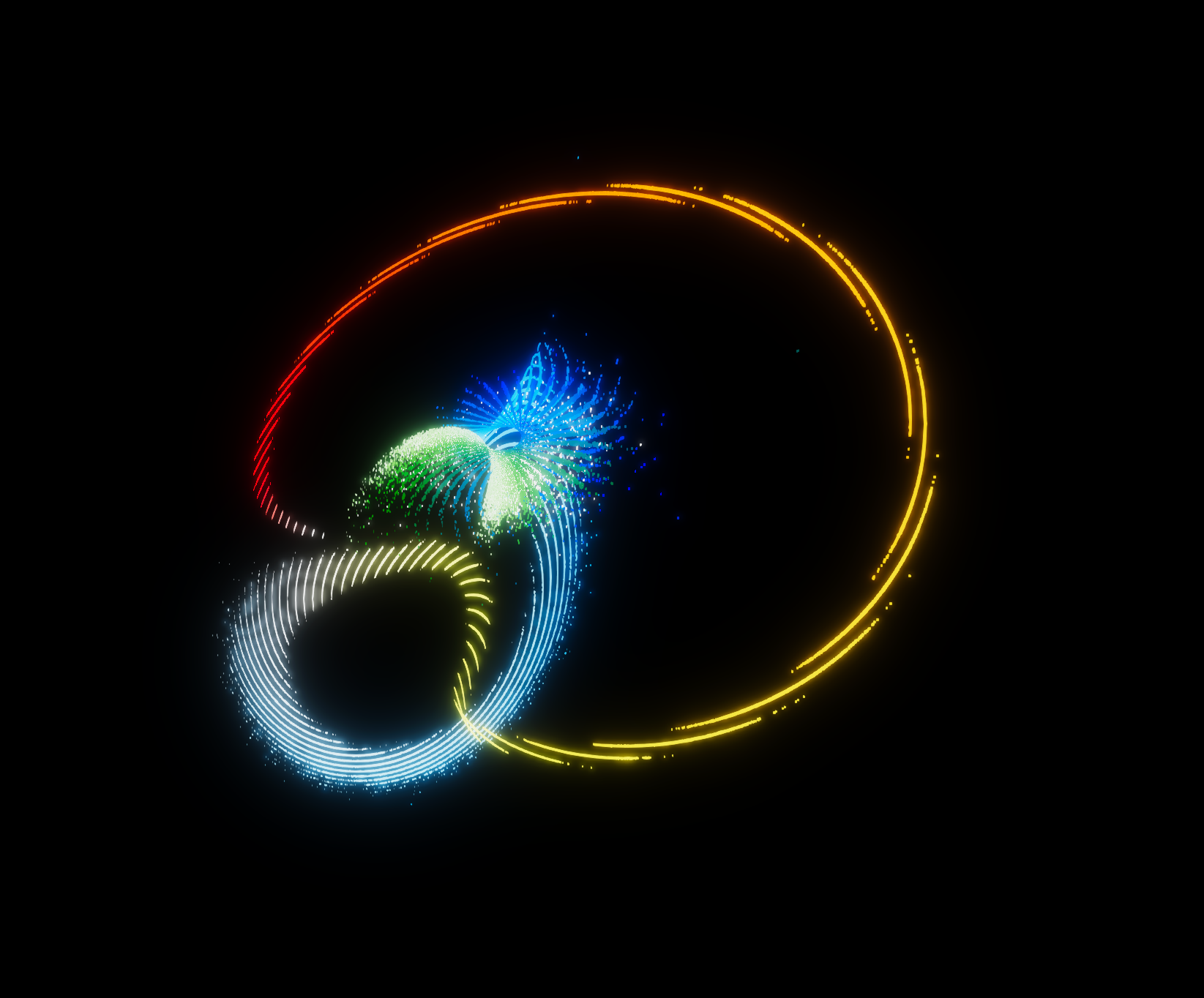
Figure 6.1: Initial state of Lorenz attractor
In this chapter, we will develop a visualization of a phenomenon called "Strange Attractor" that shows non-linear chaotic behavior by a differential equation or difference equation with a specific state using Unity and GPU arithmetic.
The sample in this chapter is "Strange Attractors" from
https://github.com/IndieVisualLab/UnityGraphicsProgramming3
.
A state in which the motion of a dissipative system (energy non-conservation, an unbalanced system with a specific input and opening) maintains a stable orbit over time is called an "Attractor".
Among them, the one that shows a chaotic behavior by amplifying the slight difference in the initial state with the passage of time is called "Strange Attractor".
In this chapter, I would like to take up " * 1 Lorenz Attractor" and " * 2 Thomas' Cyclically Symmetric Attractor" as the subjects .
Do you know the phenomenon called the butterfly effect? This is a word derived from the title of a lecture given by meteorologist Edward N Lorenz at the American Association for the Advancement of Science in 1972, " * 3 Does the flapping of a single Brazilian butterfly cause a tornado in Texas?"
This term describes a phenomenon in which slight differences in initial values do not always produce mathematically similar results, but are amplified chaotically and behave unpredictably.
Lorenz, who pointed out this mathematical property, published "Lorenz Attractor" in 1963.
Figure 6.1: Initial state of Lorenz attractor

Figure 6.2: Mid-term Lorenz attractor
[*1] Lorenz, E. N.: Deterministic Nonperiodic Flow, Journal of Atmospheric Sciences, Vol.20, pp.130-141, 1963.
[*2] Thomas, René(1999). "Deterministic chaos seen in terms of feedback circuits: Analysis, synthesis, 'labyrinth chaos'". Int. J. Bifurcation and Chaos. 9 (10): 1889–1905.
[*3] http://eaps4.mit.edu/research/Lorenz/Butterfly_1972.pdf
The Lorenz equation is represented by the following nonlinear ODE.
By setting p = 10, r = 28, b = 8/3 in each variable of p, r, and b in the above equation, it will behave chaotically as "Strange Attractor".
Now let's implement the Lorenz equation with a compute shader. First, define the structure you want to calculate in the compute shader.
StrangeAttractor.cs
protected struct Params
{
    Vector3 emitPos;
    Vector3 position;
    Vector3 velocity; // xyz = velocity, w = velocity coef;
    float   life;
    Vector2 size;     // x = current size, y = target size.
    Vector4 color;

    public Params(Vector3 emitPos, float size, Color color)
    {
        this.emitPos = emitPos;
        this.position = Vector3.zero;
        this.velocity = Vector3.zero;
        this.life = 0;
        this.size = new Vector2(0, size);
        this.color = color;
    }
}
Since this structure will be used universally in multiple Strange Attractors in the future, it is defined in the abstract class StrangeAttractor.cs.
Next, the Compute Buffer is initialized.
LorenzAttrator.cs
protected sealed override void InitializeComputeBuffer()
{
    if (cBuffer != null) cBuffer.Release();

    cBuffer = new ComputeBuffer(instanceCount, Marshal.SizeOf(typeof(Params)));
    Params[] parameters = new Params[cBuffer.count];
    for (int i = 0; i < instanceCount; i++)
    {
        var normalize = (float)i / instanceCount;
        var color = gradient.Evaluate(normalize);
        parameters[i] = new Params(Random.insideUnitSphere *
            emitterSize * normalize, particleSize, color);
    }
    cBuffer.SetData(parameters);
}
The abstract method InitializeComputeBuffer defined in the abstract class StrangeAttractor.cs is implemented in LorenzAttrator.cs.
Since I want to adjust the gradation, emitter size, and particle size in Unity's inspector, initialize the Params structure with the gradient, emitterSize, and particleSize exposed in the inspector, and setData to the ComputeBuffer variable, cBuffer.
This time, I want to apply the velocity vector by delaying it little by little in the order of particle id, so I add the gradation color in order of particle id.
In "Strange Attractor", the initial position is greatly related to the subsequent behavior depending on the thing, so I would like you to try various initial positions, but in this sample, the sphere is the initial shape.
Then pass the LorenzAttrator variables p, r, b to the compute shader.
LorenzAttrator.cs
[SerializeField, Tooltip("Default is 10")]
float p = 10f;
[SerializeField, Tooltip("Default is 28")]
float r = 28f;
[SerializeField, Tooltip("Default is 8/3")]
float b = 2.666667f;

private int pId, rId, bId;
private string pProp = "p", rProp = "r", bProp = "b";

protected override void InitializeShaderUniforms()
{
    pId = Shader.PropertyToID(pProp);
    rId = Shader.PropertyToID(rProp);
    bId = Shader.PropertyToID(bProp);
}

protected override void UpdateShaderUniforms()
{
    computeShaderInstance.SetFloat(pId, p);
    computeShaderInstance.SetFloat(rId, r);
    computeShaderInstance.SetFloat(bId, b);
}
Next, initialize the state of particles at the time of emission on the compute shader side.
LorenzAttractor.compute
#pragma kernel Emit
#pragma kernel Iterator

#define THREAD_X 128
#define THREAD_Y 1
#define THREAD_Z 1
#define DT 0.022

struct Params
{
    float3 emitPos;
    float3 position;
    float3 velocity; //xyz = velocity
    float  life;
    float2 size;     // x = current size, y = target size.
    float4 color;
};

RWStructuredBuffer<Params> buf;

[numthreads(THREAD_X, THREAD_Y, THREAD_Z)]
void Emit(uint id : SV_DispatchThreadID)
{
    Params p = buf[id];
    p.life = (float)id * -1e-05;
    p.position = p.emitPos;
    p.size.x = 0.0;
    buf[id] = p;
}
Initialization is performed by the Emit method. p.life manages the time since the generation of particles, and provides a small delay for each id at the time of the initial value.
This is to easily prevent the particles from drawing the same trajectory all at once. Also, since the gradation color is set for each id, it is useful for making the color look beautiful.
Here, the particle size p.size is set to 0 at the initial stage, but this is to make the particles invisible at the moment of occurrence to make the balloon natural.
Next, let's look at the iteration part.
LorenzAttractor.compute
#define DT 0.022

// Lorenz Attractor parameters
float p;
float r;
float b;

// The arithmetic part of the Lorenz equation.
float3 LorenzAttractor(float3 pos)
{
    float dxdt = (p * (pos.y - pos.x));
    float dydt = (pos.x * (r - pos.z) - pos.y);
    float dzdt = (pos.x * pos.y - b * pos.z);
    return float3(dxdt, dydt, dzdt) * DT;
}

[numthreads(THREAD_X, THREAD_Y, THREAD_Z)]
void Iterator(uint id : SV_DispatchThreadID)
{
    Params p = buf[id];
    p.life.x += DT;
    // Clamp the vector length of the velocity vector from 0 to 1 and multiply it by the size to make the start look natural.
    p.size.x = p.size.y * saturate(length(p.velocity));
    if (p.life.x > 0)
    {
        p.velocity = LorenzAttractor(p.position);
        p.position += p.velocity;
    }
    buf[id] = p;
}
The LorenzAttractor method above is the arithmetic part of the "Lorenz equation". The velocity vector of x, y, z with a small amount of delta time is calculated, and finally the delta time is multiplied to derive the amount of movement.
From experience, when performing derivative operations related to the shape in the compute shader, it is better to use a fixed value delta time independent of the frame rate difference instead of sending the delta time from Unity to maintain a stable shape.
This is because if the frame rate drops too much, the value of Unity's Time.deltaTime may become too large for differential operations. The larger the delta width, the rougher the calculation result will be compared to the previous one.
Another reason is that, depending on the equation, the "Strange Attractor" may completely converge or diverge infinitely depending on how the delta time is taken.
For these two reasons, DT is using the predefined ones this time.
Next, I would like to implement the "Thomas' Cyclically Symmetric Attractor" announced by biologist René Thomas.
It is not affected by the initial value, it becomes stable over time, and the shape is very unique.
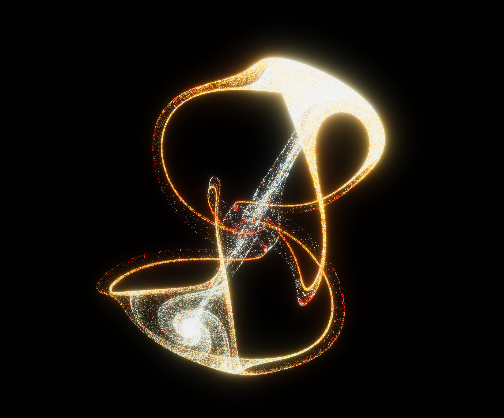
Figure 6.3: Thomas' Cyclically Symmetric Attractor Stable Period
The equation is represented by the following nonlinear ODE.
In the variable b of the above equation, if it is set as b \ simeq 0.208186, it behaves chaotically as "Strange Attractor", and if it is set as b \ simeq 0, it floats in space.
Now let's implement the "Thomas' Cyclically Symmetric equation" with a compute shader.
Since there is a part in common with the implementation of "Lorenz Attractor" mentioned above, the parameter structure and procedural part are inherited and only the necessary part is taken up.
First, override the color and initial position on the CPU side.
ThomasAttractor.cs
protected sealed override void InitializeComputeBuffer()
{
    if (cBuffer != null) cBuffer.Release();

    cBuffer = new ComputeBuffer(instanceCount, Marshal.SizeOf(typeof(Params)));
    Params[] parameters = new Params[cBuffer.count];
    for (int i = 0; i < instanceCount; i++)
    {
        var normalize = (float)i / instanceCount;
        var color = gradient.Evaluate(normalize);
        parameters[i] = new Params(Random.insideUnitSphere *
            emitterSize * normalize, particleSize, color);
    }
    cBuffer.SetData(parameters);
}
This time, in order to make the colors look beautiful, the initial position is a sphere with a mantle-like gradation color from the inside to the outside.
Next, let's look at the compute shader methods at the time of emission and iteration.
ThomasAttractor.compute
//Thomas Attractor parameters
float b;

float3 ThomasAttractor(float3 pos)
{
    float dxdt = -b * pos.x + sin(pos.y);
    float dydt = -b * pos.y + sin(pos.z);
    float dzdt = -b * pos.z + sin(pos.x);
    return float3(dxdt, dydt, dzdt) * DT;
}

[numthreads(THREAD_X, THREAD_Y, THREAD_Z)]
void Emit(uint id : SV_DispatchThreadID)
{
    Params p = buf[id];
    p.life = (float)id * -1e-05;
    p.position = p.emitPos;
    p.size.x = p.size.y;
    buf[id] = p;
}

[numthreads(THREAD_X, THREAD_Y, THREAD_Z)]
void Iterator(uint id : SV_DispatchThreadID)
{
    Params p = buf[id];
    p.life.x += DT;
    if (p.life.x > 0)
    {
        p.velocity = ThomasAttractor(p.position);
        p.position += p.velocity;
    }
    buf[id] = p;
}
The ThomasAttractor method becomes the arithmetic part of the "Thomas' Cyclically Symmetric equation".
Also, unlike LorenzAttrator, the implementation at Emit is set from the initial size to the target size because I want to show the initial position this time.
Others have almost the same implementation.
In this chapter, we introduced an example of implementing "Strange Attractor" on GPU using a compute shader.
There are various types of "Strange Attractor", and even in the implementation, it shows chaotic behavior with relatively few operations, so it may be a useful accent in graphics as well.
There are many other types, such as a two-dimensional motion called " * 4 Ueda Attractor" and a spin motion like " * 5 Aizawa Attractor", so if you are interested, please try it.
[*4] http://www-lab23.kuee.kyoto-u.ac.jp/ueda/Kambe-Bishop_ver3-1.pdf
[*5] http://www.algosome.com/articles/aizawa-attractor-chaos.html